

In several previous posts I investigated advantage play against loss rebates. These include two posts on Don Johnson (post 1, post 2) as well as this post on baccarat loss rebates and these two posts (post 1, post 2) on roulette loss rebates. My methodology has been to run a bunch of simulations for various win and loss-exit points to find those exit points that maximize the player’s return. By simulating the actual game, these results produce numbers that are very accurate, within the limitations of the size of the simulation. With all this brute force number crunching, some part of me knew there was an easier way to solve this using a theoretical approach.
Skip back to my third year of graduate school (1981). In the Spring semester of that year, I audited a course called “Stochastic Processes.” By auditing I mean I sat in class, but took no notes, did no homework, owned no textbook and took no tests. My degree was in “Algebraic Number Theory” and this information was far afield from my main studies. I’ve known this subject matter directly applies to loss rebates for some time, but without a book or notes to look at, I’ve chosen the surefire shortcut of number crunching. With the recent publicity surrounding Don Johnson's exploitation of loss rebates, I set out to resurrect these old theorems and figure out how to use them. It turned out to be remarkably easy to find the critical information with a Google search.
In the book An Introduction to Stochastic Modeling, by Howard M. Taylor and Samuel Karlin, 3rd edition, 1998 by Academic Press, I found these two theorems (click on the images to get larger, easier to read versions):


These look complicated, no doubt. But, as it turns out, they are perfectly suited for our purposes. With about 5 minutes of scratch work, I wrote out the following theorem that rephrased these results into terms that allow them to be applied to loss rebates:
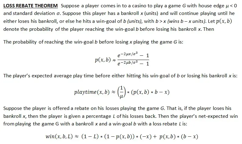
I couldn't figure out how to get these formulas into a blog post, hence the hard to read image above. Click on the image above and you will get a full size version.
The reader may wonder at using the “approximately equal” symbol as opposed to simple equality. The reason for this is that in Theorem 4.1 and 4.2, the underlying distribution was assumed to be normal whereas casino games have non-normal discrete distributions. A proper loss rebate theorem would quantify the precise nature of "approximately equal." Please forgive me for not taking the dive into those murky waters.
The issue of non-normal distributions gives some practical limitations to the accuracy of these formulas for modeling casino games. For example, they work much better on baccarat and blackjack than on video poker and slots. These formulas also perform better when b is much larger than x, so they don’t work well for modest win-goals with a large player bankroll.
My purpose in this theoretical effort is to be able to quickly determine the values of b and x that maximize the APs return for a given game G and loss rebate L. Towards that end, I first wrote a computer program to output the values obtained from the three formulas given in the Loss Rebate Theorem for any values of b and x. For any particular situation, I modified the program with some additional logic to have it solve the problem of maximizing the win for the AP, that is, finding the best possible b and x. My program then output the player’s loss-exit point, his win-exit point, his probability of winning, his expected playtime and his win amount. It took about an hour to write the program and a matter of milliseconds to complete each computation.
Sometimes I want to kick myself for being intellectually lazy.
Example 1. Don Johnson, Blackjack.
In this example I consider Don Johnson’s assault on Atlantic City. The game he played was blackjack, with μ = -0.0029036, σ = 1.1417. His loss rebate was L = 20% and his wagering unit was $100,000. I re-wrote my program to find the values of x and b that maximized Johnson’s return:
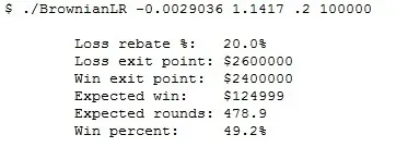
The final number in this output (win percent) gives the percentage of times that Johnson will reach his win exit point before reaching his loss exit point.
In this post, I determined by simulation that with a quit loss of $2,750,000 and quit win of $2,200,000, Don Johnson will have an expected win of $125,209 with 453 expected rounds. These numbers are remarkably close to what was predicted in theory.
Example 2. Baccarat, Loss Rebate = 18%.
Here is another example. Suppose the game is baccarat and that the player is making only Banker bets of size $100,000. In this case, μ = -0.010579, σ = 0.927372, L = 18%, with wagering unit = $100,000:
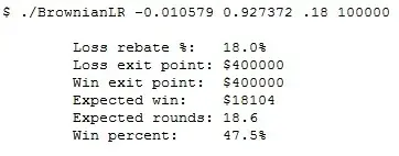
Compare these results with those given in this post, where simulation gave a quit loss point of $450,000 and a quit win point of $360,000. In the case of simulation, the player won $18,050 in an average of 18.7 hands. Theory gives a player win of $18,104 in 18.6 hands. Once again, these results are remarkably close to each other. The distribution for baccarat is quite “Normal” (it's about as normal as a three-event discrete distribution can be).
Simulation will remain the main tool for games like video poker, or for wagers like straight-up bets on roulette. In particular, the recent 100% rebate on losses promotion at Revel was best served by simulation.
Casino gambling is a perfect testing ground for the match between theory and reality. It is about time I caught up to the late-20th century when it comes to loss rebate analysis for games like blackjack and baccarat.
[Acknowledgement. I would like to thank Michael Shackleford for bringing the distribution issues when using these results for video poker to my attention. He also provided the values for μ and σ I used in Example #1 in this article.]
