Loss rebate analysis has been a common topic in this blog. There's a good reason: it is one of the top advantage play opportunities worldwide. Exploiting loss rebates is how Don Johnson crushed Atlantic City. Previously, my key theoretical result was when I proved the Loss Rebate Theorem and gave a spread sheet to help work with that theorem. But, I had never fully solved the problem by finding closed form solutions for the win-quit and loss-quit points. Today while walking my dog, an idea occurred to me about how I might completely solve the loss rebate problem. After a couple of hours of computation, the method worked! This post presents this "second" Loss Rebate Theorem, its proof, a spread sheet and an example. My dog is very proud of me.
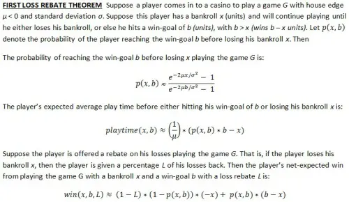
To remind you, here is the original Loss Rebate Theorem (click on the image to make it larger):

The First Loss Rebate Theorem (LRT1) gives the player’s net-expected win, assuming the values x (the player’s bankroll) and b (the players win-goal) are fixed. I used this theorem in practice by writing a small computer program that looped over a lot of different values of x and b until I found the ones that gave the largest value for win(x,b,L). The question that LRT1 did not answer is: what specific values of x and b maximize win(x,b,L)?
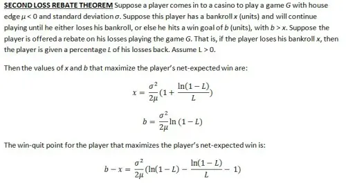
In retrospect, the methodology to answer this question is quite trivial. To maximize a function of two variables, take the partial derivatives with respect to each variable, set both partial derivatives equal to zero, and solve the simultaneous equations. As I found out during the computation, it is simply good luck that these two equations can actually be solved in closed form. A bit of care needs to be taken that the result is actually a maximum (not a minimum or a saddle point), but in our situation it is intuitively obvious that this is the case.
So here it is, the Second Loss Rebate Theorem (LRT2) (click on the image to make it larger):

Here is the derivation of these formulas, if you want to see my work. I re-wrote this once, but not twice, so it may be tough to follow: LRT_Proof
Here is a spread sheet you can (should!) download that allows you to easily use LRT1 and LRT2: Loss_Rebate_Theorem_Full_Solution
I am guessing that James Grosjean already knows and has proved LRT1 and LRT2, but I have not seen either if he has. I certainly expect that Don Johnson used this theorem when he attacked Atlantic City. He claimed to have "Ph.D. mathematicians" working for him (not me!). Theorems LRT1 and LRT2 are elegant and easy to use. No simulations needed. Moreover, the values of x and b produced by LRT2 can be plugged straight into the formulas in LRT1. Together they give us the win-quit point, loss-quit point, probability of winning, expected play time and the net-expected win. What else could we want?
Here is an example. Consider Don Johnson’s efforts in Atlantic City. He played a six-deck shoe game with a loss-rebate of 20%. In this case,
- μ = -0.0029036
- σ = 1.1417
- L = 0.20
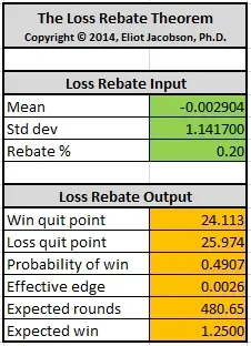
Here are the results analyzing Don Johnson when LRT1 and LRT2 are used together in the spread sheet I created (the link for downloading this spreadsheet is given above):

We see that with a $100,000 wager,
- Don Johnson should quit after winning $2,411,300.
- Don Johnson should quit after losing $2,597,400.
- The probability of hitting the win-quit point in any given session is 49.07%.
- Don Johnson was playing with an effective edge over the house of about 0.26%.
- The number of expected rounds to reach a quit point is 481.
- The expected win per session for Don Johnson was $125,000.
Here are the results I obtained from a large Monte Carlo simulation of Don Johnson (see this post). Note that I incremented the bankrolls by $250k segments in this simulation, hence did not consider a quit-loss point of $260,000. In my opinion, LRT1 and LRT2 performed very well compared to this simulation.
- Quit-win = $2,200,000.
- Quit-loss = $2,750,000.
- Expected rounds = 453.
- Expected win per session: $125,209
[ Note. I would like to thank "puzzlenut" who inspired me to think about this problem again in this thread. ]


